Someone on the team asked a simple question: "What was our Q3 revenue?" The RAG pipeline pulled 127,000 tokens of context. Earnings transcripts, board decks, internal forecasts, analyst reports. The model read all of it and returned the wrong number.
Not a hallucination exactly. It found a Q3 figure. But it was from a draft forecast, not the final audited report. Both documents were sitting in the context window, and the model picked the wrong one. The correct answer was buried in the middle of a 94-page earnings document, surrounded by dozens of other chunks that mentioned Q3 in passing.
We had been running at 128K context windows for three months at that point. The bill was $2,400 per day in inference costs. And the accuracy on financial questions, the ones that actually mattered, was sitting at 81%.
So we ran an experiment. We rebuilt the retrieval pipeline to be aggressive about what goes into the context window. Metadata pre-filtering, cross-encoder re-ranking, and dynamic context budgets that scale with query complexity. The result was a system that typically sends between 8K and 32K tokens of context instead of 128K.
Costs dropped from $2,400 to $890 per day. A 63% reduction. And accuracy on the same benchmark set went from 81% to 88%. Less context, better answers, lower cost. That is what context window management as a cost lever looks like in practice.
This post is the full breakdown of how we got there.
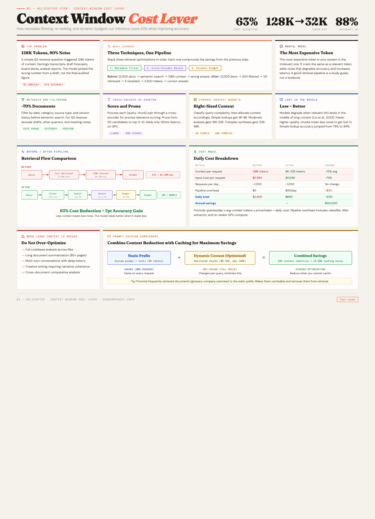
For a visual breakdown of the before/after pipeline, see the Context Window Cost Lever infographic.
Before vs After: The Full Picture#
| Metric | Before | After |
|---|---|---|
| Context Size | 128K tokens | 8K-32K tokens |
| Daily Cost | $2,400/day | $890/day |
| Accuracy | 81% | 88% |
| Latency (p50) | 4.2 seconds | 1.8 seconds |
| Technique Used | Raw semantic search | Metadata filter + cross-encoder re-rank + dynamic budget |
The most expensive token in your system is the irrelevant one. It costs the same as a relevant token, adds noise that degrades accuracy, and increases latency for every request that carries it.
Table of Contents#
- How does context window size affect inference cost?
- The three optimization techniques
- The counter-intuitive finding: less context means better answers
- Prompt caching as a complementary strategy
- Implementation guide: building a context-efficient RAG pipeline
- Cost modeling: how to estimate savings for your workload
- When you actually need large context windows
- Results at a glance
- FAQ
How Does Context Window Size Affect Inference Cost?#
This part is straightforward but worth making explicit because I have watched teams skip over it.
LLM inference pricing is denominated in tokens. Every major provider charges per input token and per output token separately. When you send 128K tokens of context to the model, you pay for 128K input tokens. When you send 32K, you pay for 32K. The relationship is linear. Four times the context, four times the cost.
Here is the math on Claude Sonnet 4.6, which is what we were running:
| Context size | Input cost per request | Daily cost (1,000 requests) |
|---|---|---|
| 128K tokens | $0.384 | $384 |
| 64K tokens | $0.192 | $192 |
| 32K tokens | $0.096 | $96 |
| 8K tokens | $0.024 | $24 |
Those are just the input token costs. Output tokens add on top. But the important thing to see is the linear scaling. There is no volume discount on context window size. Every token you send costs the same whether you send a hundred or a hundred thousand.
For our system, the total daily cost included output tokens, prompt caching overhead, and some retry logic. The $2,400 to $890 drop reflected all of those together. But the dominant factor was input tokens. We were sending roughly 75% fewer tokens per request on average.
The other cost dimension people forget about is latency. Larger context windows take longer to process. Time-to-first-token scales with input length because the model has to attend to every token in the prompt before it can start generating. Our p50 latency dropped from 4.2 seconds to 1.8 seconds, which mattered for the internal tool we were building. Users notice when an answer takes four seconds.
Key takeaway: Context window size drives inference cost linearly. Four times the context means four times the cost. There is no volume discount on token count, and larger windows also increase latency because the model must attend to every input token before generating output.
There is a deeper architectural point here too. If you are building agentic systems that make multiple LLM calls per user request, the context window cost multiplies across every call in the chain. An orchestrator that calls three sub-agents, each with their own context, means your effective cost is three times whatever a single call costs. Tightening the context at each stage compounds the savings.
The Three Optimization Techniques#
We did not invent any of these. They are well-known in the information retrieval literature. What we did was stack them together in a specific order and measure the combined effect carefully.
Technique 1: Metadata Pre-Filtering#
This is the simplest one and probably has the highest impact-to-effort ratio of anything in this post.
Before you do any semantic search, filter the document set using structured metadata. Date ranges, document categories, source labels, version flags. The goal is to eliminate irrelevant documents before they ever touch the embedding similarity calculation.
Going back to the Q3 revenue example: the question "What was our Q3 revenue?" contains an implicit time constraint. Q3. The system should know which fiscal year the user means (almost always the most recent one) and filter to documents from that period before doing semantic retrieval.
Here is what our filter pipeline looks like:
def apply_metadata_filters(query: str, documents: list[Document]) -> list[Document]:
    """
    Pre-filter documents based on structured metadata
    extracted from the query.
    """
    filters = extract_query_filters(query)

    filtered = documents
    if filters.date_range:
        filtered = [
            d for d in filtered
            if d.metadata.date >= filters.date_range.start
            and d.metadata.date <= filters.date_range.end
        ]
    if filters.categories:
        filtered = [
            d for d in filtered
            if d.metadata.category in filters.categories
        ]
    if filters.source_types:
        filtered = [
            d for d in filtered
            if d.metadata.source_type in filters.source_types
        ]
    if filters.version_filter == "final_only":
        filtered = [
            d for d in filtered
            if d.metadata.is_final is True
        ]

    return filtered
The extract_query_filters function is a lightweight classifier. We use a small model (Haiku) to parse the user query into structured filter fields. It costs almost nothing per call and runs in under 100 milliseconds. The prompt is roughly: "Given this user question, extract any implied date ranges, document categories, and version requirements. Return JSON."
For the Q3 revenue case, this filter step eliminated about 80% of the document corpus before semantic search even started. Draft documents were excluded. Documents from other quarters were excluded. Meeting notes that happened to mention revenue in passing were excluded.
Key takeaway: Metadata pre-filtering delivers approximately 70% reduction in candidate documents before any semantic search runs. It is the highest impact-to-effort technique in this stack. For our system, it alone accounted for 40% of the total cost savings.
The important design decision here: metadata has to exist and be clean. This means you need to invest in your ingestion pipeline. Every document that enters the system needs reliable metadata, date, category, source type, version status. If your metadata is noisy, the filtering is noisy. Garbage in, garbage out, as always.
We tag documents at ingestion time using a combination of file path conventions (anything under /earnings/final/ is a final earnings document), extraction rules (pull the date from the document header), and a small classification model that labels ambiguous documents.
Technique 2: Cross-Encoder Re-Ranking#
After metadata filtering and semantic search, you have a set of candidate chunks. Maybe 40 or 50 of them, ranked by embedding cosine similarity. The problem is that bi-encoder embeddings are fast but not precise. They are good at finding documents that are roughly relevant but bad at distinguishing "somewhat related" from "exactly what was asked."
Cross-encoder re-ranking fixes this. Instead of comparing query and document embeddings independently, a cross-encoder processes the query and each candidate chunk together as a single input. It outputs a relevance score that is much more accurate than cosine similarity.
The trade-off is speed. A cross-encoder has to run inference for every (query, chunk) pair. If you have 50 candidates, that is 50 forward passes. On a model like cross-encoder/ms-marco-MiniLM-L-6-v2, each pass takes about 2-3 milliseconds on a GPU. So 50 candidates cost roughly 120 milliseconds. That is the number I mentioned in the LinkedIn post.
120 milliseconds sounds like a lot if you are used to thinking about web response times. But remember what it is replacing: sending all 50 chunks to the LLM costs you 50 times the chunk size in input tokens and adds seconds of latency. The re-ranker lets you prune from 50 chunks down to the top 5 or 10, which cuts your context by 80-90% at a cost of 120 milliseconds of re-ranking time.
Here is how we use it:
from sentence_transformers import CrossEncoder

reranker = CrossEncoder("cross-encoder/ms-marco-MiniLM-L-6-v2")

def rerank_and_prune(
    query: str,
    chunks: list[Chunk],
    top_k: int = 10,
    min_score: float = 0.3,
) -> list[Chunk]:
    """
    Re-rank chunks using cross-encoder, then prune
    to top_k results above the minimum score threshold.
    """
    pairs = [(query, chunk.text) for chunk in chunks]
    scores = reranker.predict(pairs)

    scored_chunks = sorted(
        zip(chunks, scores),
        key=lambda x: x[1],
        reverse=True,
    )

    return [
        chunk for chunk, score in scored_chunks[:top_k]
        if score >= min_score
    ]
Two parameters matter here. top_k controls how many chunks survive. min_score is a quality floor. If re-ranking reveals that even the best candidate has a score below 0.3, you probably do not have relevant documents at all, and the system should say so rather than hallucinate from weak context.
We settled on top_k=10 and min_score=0.3 after testing on about 500 question-answer pairs. Your thresholds will be different depending on your corpus and use case. The point is to tune them empirically, not to guess.
Key takeaway: A cross-encoder re-ranker adds roughly 120 milliseconds of latency but eliminates 80-90% of candidate chunks. It costs orders of magnitude less than sending those extra chunks to the LLM, and the relevance scoring is far more precise than cosine similarity alone.
One subtlety that took us a while to learn: the re-ranker's effectiveness depends heavily on chunk size. If your chunks are too large (say, entire document sections of 2,000 tokens), the cross-encoder struggles because it is attending to a lot of irrelevant text within each chunk. If chunks are too small (50 tokens), it lacks enough context to judge relevance. We found that 300 to 500 token chunks with 50-token overlaps worked best for our financial documents.
Technique 3: Dynamic Context Budgets#
Not every query needs the same amount of context. "What was Q3 revenue?" is a lookup. The answer is a single number in a specific document. Sending 32K tokens of context for that is wasteful. On the other hand, "Compare our revenue growth trajectory across Q1 through Q4 and identify which product lines drove the acceleration" genuinely needs a lot of context because the answer requires synthesizing information from multiple documents.
Dynamic context budgets solve this by classifying queries into complexity tiers and allocating context accordingly.
We use three tiers:
| Tier | Context budget | Example queries |
|---|---|---|
| Simple lookup | 4K-8K tokens | "What was Q3 revenue?", "Who is our CFO?" |
| Moderate analysis | 16K-32K tokens | "Summarize key risks from the 10-K", "What changed between Q2 and Q3 guidance?" |
| Complex synthesis | 32K-48K tokens | "Compare product line performance across all quarters and identify trends", multi-document analysis |
The classifier is a small prompted model call. We feed it the user query and ask it to categorize into one of the three tiers, returning a JSON object with the tier and a confidence score. If confidence is below 0.7, we default to the moderate tier. The classifier prompt includes a few examples of each tier to anchor it.
CLASSIFIER_PROMPT = """Classify this query into a complexity tier.

Tiers:
- simple: Fact lookup, single data point, yes/no question
- moderate: Summary, comparison of 2-3 items, trend in one dimension
- complex: Multi-document synthesis, cross-quarter analysis, causal reasoning

Examples:
- "What was Q3 revenue?" -> simple
- "Summarize the risk factors" -> moderate
- "Compare all product lines across 4 quarters" -> complex

Query: {query}

Return JSON: {"tier": "simple|moderate|complex", "confidence": 0.0-1.0}"""
The budget is not a hard cap. It is a target that controls how many chunks the retrieval pipeline returns. If re-ranking produces only 3 high-quality chunks totaling 1,500 tokens for a simple query, we do not pad it to reach 8K. The budget is an upper bound.
One thing we tried and abandoned was using the LLM itself to decide how much context it needs. This circular approach does not work well because the model cannot know what it needs without first seeing the available context. The external classifier approach is simpler and more reliable.
The combined effect of all three techniques is substantial. For the Q3 revenue question that started this whole effort, the pipeline now works like this:
- Metadata filter narrows from 12,000 documents to about 200 (Q3 dates, earnings category, final versions only)
- Semantic search retrieves the top 50 chunks from those 200 documents
- Cross-encoder re-ranking prunes to the top 5 chunks, all from the actual Q3 earnings report
- Dynamic budget classifies as "simple" and caps at 8K tokens
- Total context sent to the model: roughly 2,500 tokens
Compare that to the original pipeline, which just did semantic search across the full corpus and stuffed 128K tokens into the context. The difference in cost, latency, and accuracy is dramatic.
Key takeaway: Dynamic context budgets classify each query by complexity and allocate only the context that query type requires. Simple lookups get 4K-8K tokens. Complex synthesis tasks get 32K-48K. The budget is an upper bound, not a target. Combined with filtering and re-ranking, this pipeline sent roughly 2,500 tokens for a question that previously consumed 128K.
Less Context Means Better Answers#
This is the part that surprises people. I expected smaller context windows to be cheaper but slightly less accurate, a reasonable trade-off. Instead, accuracy went up.
The explanation comes from research on how transformer models handle long contexts. The phenomenon is called the "lost in the middle" problem, documented in a 2023 paper by Liu et al. at Stanford. Their finding: when relevant information is placed in the middle of a long context, model performance degrades significantly compared to when the same information appears at the beginning or end.
Think about what that means for RAG. When you stuff 128K tokens of context into the prompt, the relevant chunks are surrounded by dozens of semi-relevant and irrelevant chunks. The model has to figure out which ones matter. And the evidence shows that models are not great at this, especially when the answer-bearing passage lands somewhere in the middle of the sequence.
By contrast, when you send 5 high-quality chunks totaling 2,500 tokens, every chunk is relevant. There is no noise to get lost in. The model can focus entirely on the information that matters.
We measured this across 500 question-answer pairs from our financial document corpus. The results by tier:
| Metric | 128K context (before) | Optimized (after) | Change |
|---|---|---|---|
| Simple lookup accuracy | 79% | 94% | +15 pts |
| Moderate analysis accuracy | 83% | 87% | +4 pts |
| Complex synthesis accuracy | 82% | 84% | +2 pts |
| Overall accuracy | 81% | 88% | +7 pts |
The gains are largest for simple lookups, which makes sense. A simple lookup has one correct answer in one document. Sending 128K of context buries that answer in noise. Sending 2,500 tokens of well-selected context makes the answer obvious.
For complex synthesis tasks, the improvement is smaller. These tasks genuinely benefit from more context because the answer spans multiple documents. But even here, curated context beats raw context because the re-ranker has already filtered out the irrelevant chunks.
There is an analogy I keep coming back to. Imagine you are studying for an exam and someone hands you a 500-page textbook versus a 20-page study guide written by someone who already read the textbook and extracted the important parts. You will do better with the study guide, not because it contains more information, but because it contains the right information without the distraction.
That is what a good retrieval pipeline does for an LLM. It acts as the study guide author.
Key takeaway: The model is not a better reader when you give it more text. It is a better reader when you give it the right text. Our simple lookup accuracy jumped from 79% to 94% after reducing context from 128K to well-curated chunks, a 15 percentage point gain from sending less data, not more.
Prompt Caching as a Complementary Strategy#
Context window optimization and prompt caching are separate techniques that stack well together. I have written about prompt caching in detail in The Complete Guide to Prompt Caching for AI Agents and The Static-First Prompt Architecture, so I will not repeat all of that here. But the interaction between the two is worth covering.
Prompt caching works by hashing a prefix of your prompt and storing the key-value attention computations for that prefix. On subsequent requests with the same prefix, the cached computation is reused. With Anthropic's prompt caching, cached input tokens cost 90% less than uncached ones.
Here is how the two strategies combine:
Your system prompt, tool definitions, and project context are cacheable. These do not change between requests. A well-structured prompt has these static elements at the top, with cache breakpoints placed after each one. This is the layered architecture I described in the prompt caching post.
Your retrieved context is dynamic and typically not cacheable. Each query pulls different chunks, so this part of the prompt changes on every request. This is exactly why you want it to be as small as possible. The uncacheable portion of the prompt is where your per-token costs hit hardest.
The math works out favorably. Say your static prefix is 4,000 tokens (system prompt plus tool definitions) and your dynamic context is the variable part. With caching, the 4,000 token prefix costs 90% less on repeat calls. So your effective cost per request is:
cost = (4000 * $0.0003) + (dynamic_context * $0.003)
The dynamic context dominates the cost. Which means reducing the dynamic context from 128K to 8K has an outsized effect on total cost even when caching is already in play.
In our system, enabling prompt caching on top of context window optimization reduced costs by another 15-20% beyond the 63% we got from context optimization alone. The two are complementary.
Key takeaway: Context reduction and prompt caching are complementary, not competing strategies. Caching reduces the cost of static prompt elements by 90%. Context optimization reduces the dynamic, uncacheable portion. Stacking both gave us an additional 15-20% savings beyond the 63% from context reduction alone.
One practical tip: if you have documents that appear frequently across many queries (a company overview document, a glossary of terms, a standard disclaimer), consider promoting them to the static context layer rather than retrieving them dynamically each time. This makes them cacheable. We moved five "always relevant" documents into the system prompt prefix, which cost us about 2,000 additional cached tokens but eliminated those documents from the retrieval pipeline entirely.
Implementation Guide#
Here is a step-by-step guide to building a context-efficient RAG pipeline. I am assuming you already have a basic RAG system with document ingestion, embedding, and retrieval. The goal is to add the three optimization layers on top.
Step 1: Enrich Your Document Metadata#
Before you can filter on metadata, you need to have it. Go through your ingestion pipeline and add structured fields to every document:
- Date: When was the document created or published? Use the most specific date available.
- Category: What type of document is this? (earnings report, meeting notes, product spec, legal filing, etc.)
- Source type: Where did this come from? (internal, external, regulatory, user-generated)
- Version status: Is this a draft or a final version?
- Entities: What companies, products, or people does this document mention?
If you have a large existing corpus without metadata, you can backfill using a classification model. We used Haiku to classify and tag about 50,000 documents at a cost of roughly $15. It is not perfect, but 90% accurate metadata is dramatically better than no metadata.
Step 2: Build the Query Filter Extractor#
Write a prompt that takes a user query and outputs structured filter criteria. Keep it simple. The extractor does not need to understand the query deeply. It just needs to identify any explicit or implicit constraints.
Test it on a sample of 50-100 real queries from your system. Check that the extracted filters make sense. Common failure modes: extracting filters that are too aggressive (filtering out relevant documents), not extracting implicit time constraints ("last quarter" should map to a date range), and not handling ambiguous queries gracefully.
Step 3: Integrate a Cross-Encoder Re-Ranker#
Install sentence-transformers and load a cross-encoder model. ms-marco-MiniLM-L-6-v2 is a good starting point. It is small, fast, and accurate enough for most use cases.
Place the re-ranker after your semantic search step. Feed it (query, chunk) pairs and sort by score. Start with top_k=10 and min_score=0.3, then tune based on your evaluation set.
Measure the re-ranking latency. If it is above 200 milliseconds, you are probably passing too many candidates. Reduce the number of chunks coming out of semantic search.
Step 4: Build the Query Complexity Classifier#
This is the simplest component. A few-shot prompt to a fast model (Haiku or equivalent) that classifies queries into your defined tiers. Map each tier to a context budget.
The classifier adds one LLM call per query. In practice this costs less than a tenth of a cent and takes under 200 milliseconds. The savings from allocating the right context budget far outweigh this overhead.
Step 5: Wire It Together#
The pipeline should execute in this order:
- Query comes in
- Classifier determines complexity tier and context budget (can run in parallel with step 3)
- Filter extractor parses metadata constraints
- Apply metadata filters to document corpus
- Run semantic search on filtered corpus
- Re-rank results with cross-encoder
- Prune to top-k within the context budget
- Assemble prompt and call the LLM
Steps 2 and 3 can run in parallel because they are independent. Steps 4 through 7 are sequential.
Step 6: Build an Evaluation Set#
You cannot tune this pipeline without a ground truth evaluation set. Create 200-500 question-answer pairs covering all your complexity tiers. For each pair, include:
- The question
- The correct answer
- The document(s) that contain the answer
- The complexity tier
Run the pipeline against this evaluation set after every change. Track accuracy, cost, and latency as your three primary metrics.
Cost Modeling#
Here is a framework for estimating what context window optimization will save for your specific workload.
Step 1: Measure Your Current State#
Pull your LLM usage data for the past 30 days. You need:
- Total input tokens per day (from your API dashboard or billing)
- Average input tokens per request (total divided by request count)
- Request volume per day
- Current accuracy (if you have an evaluation set, run it)
Step 2: Estimate Your Reduction#
This depends on your current context usage pattern. Some rough benchmarks from our experience and from talking to other teams:
| Current state | Likely reduction | Notes |
|---|---|---|
| Stuffing full documents | 70-90% | You are sending way too much |
| Using top-50 chunks | 60-80% | Re-ranking will cut this significantly |
| Using top-20 chunks | 40-60% | Metadata filtering adds the most value here |
| Already using top-10 chunks | 10-30% | Dynamic budgets help for simple queries |
Step 3: Calculate Savings#
daily_savings = current_daily_cost * reduction_percentage
monthly_savings = daily_savings * 30
annual_savings = daily_savings * 365
For our case: $2,400 * 0.63 = $1,510 per day. That is $45,300 per month, or about $551,000 per year. At that scale, a two-week engineering investment to build the pipeline paid for itself in the first week of operation.
Step 4: Factor in New Costs#
The optimization pipeline adds some costs:
- Query classifier: ~$0.001 per query (Haiku call)
- Filter extractor: ~$0.001 per query (Haiku call)
- Re-ranker inference: Compute cost for running the cross-encoder, roughly $0.0001 per query if running on GPU
- Infrastructure: If you deploy a re-ranker model, you need a GPU instance or a serverless GPU endpoint
For us, the new costs totaled about $30 per day. Against $1,510 in savings, that is a rounding error.
Break-Even Analysis#
If your daily inference spend is under $50, the engineering effort to build this pipeline may not be worth it. The savings are real but small in absolute terms. If you are spending $200 or more per day on inference, this becomes one of the highest-ROI infrastructure investments you can make.
When You Actually Need Large Context Windows#
I do not want to leave the impression that large context windows are always wasteful. There are legitimate use cases where you need them.
Codebase analysis. When an AI coding agent needs to understand the relationships between multiple files, you genuinely need to fit several files into context simultaneously. This is one of the core ideas behind tools like Claude Code. The LLM Wiki Pattern is relevant here, it describes how to build personal knowledge bases that feed into LLM context.
Long document summarization. If the task is "summarize this 80-page legal agreement," you need to read the whole thing. There is no retrieval shortcut because the answer is the entire document.
Multi-turn conversation with extensive history. Chat applications where the model needs to reference things said 50 turns ago require large context to maintain coherence.
Creative writing. Generating a consistent 10,000-word story requires the model to hold the whole narrative in context to maintain character consistency and plot coherence.
Comparative analysis across many documents. Some tasks require the model to hold 15 documents in mind simultaneously to identify patterns across all of them.
The common thread is that these are tasks where the information need is genuinely broad. You need most or all of the input to produce the output. For tasks like that, optimization looks different. You focus on prompt caching (to amortize the cost of the large context) and batching (to amortize the cost across multiple outputs), rather than trying to shrink the context.
The question to ask is: "Can I identify the specific passages the model needs before sending the query?" If yes, you have a retrieval problem and context optimization helps enormously. If no, you have a comprehension problem and you need the full context.
In my experience, about 70% of production RAG queries are retrieval problems. People think they need full-document comprehension, but what they actually need is a well-identified passage plus enough surrounding context to interpret it correctly. Distinguishing between these two cases is one of the highest-value analytical exercises you can do when designing a RAG system.
Practical Lessons from Production#
A few things we learned the hard way.
Monitor context utilization, not just cost. We built a dashboard that tracks the ratio of tokens used to tokens available (the context budget). If the pipeline consistently uses less than 50% of the allocated budget, the budget is too high. If it consistently hits the ceiling, the budget is too low. This feedback loop lets you tune the tier boundaries over time.
Chunk overlap matters more than you think. When we first set up the re-ranker, we were getting duplicate information in adjacent chunks because our overlap was too large. The re-ranker would score both chunks highly because they both contained the relevant passage. We reduced overlap from 100 tokens to 50 tokens and added a deduplication step that checks for high text similarity between selected chunks.
The filter extractor needs guardrails. In early testing, the filter extractor would sometimes apply overly aggressive date filters that excluded the correct document. A question like "How has our revenue trended?" has an implicit "over the past several quarters" time range, but the extractor initially narrowed it to the most recent quarter. We added a rule: if the query implies a trend or comparison, expand the date range to the past 12 months.
Re-ranker scores are not calibrated across queries. A score of 0.8 on one query does not mean the same thing as 0.8 on another query. We learned to use relative ranking (top-k) as the primary selection mechanism and the absolute score threshold (min_score) only as a safety net to catch queries with no relevant documents.
Start with metadata filtering alone. If you are looking for a quick win, skip the re-ranker and dynamic budgets initially. Just add good metadata to your documents and filter before retrieval. We saw a 40% cost reduction from metadata filtering alone. The re-ranker and dynamic budgets added the remaining improvement, but the first step got us the majority of the value.
FAQ#
Does context window optimization conflict with prompt caching?#
No. The two strategies are complementary. Prompt caching reduces the cost of the static prefix (system prompt, tool definitions, project context). Context window optimization reduces the cost of the dynamic portion (retrieved chunks). Applying both gives you the best overall cost reduction. I cover the interaction in detail in The Complete Guide to Prompt Caching for AI Agents.
What if my documents do not have good metadata?#
You can bootstrap metadata using a classification model. We used Haiku to tag 50,000 documents with category, date, and source type at a cost of about $15. The accuracy was roughly 90%, which is good enough for filtering purposes. Over time you can improve the metadata through manual correction and better ingestion rules.
How much does the cross-encoder re-ranker add to latency?#
About 120 milliseconds for 50 candidate chunks on a GPU, using the ms-marco-MiniLM-L-6-v2 model. On CPU, it is closer to 500 milliseconds. If latency is critical, you can reduce the number of candidates passed to the re-ranker (from 50 to 20, for example) or use a smaller model.
Can I use the LLM itself as the re-ranker instead of a separate model?#
You can, and some teams do. The LLM will generally produce better relevance judgments than a small cross-encoder. But the cost defeats the purpose. You are trying to reduce the tokens you send to the LLM, and using the LLM to decide which tokens to send creates a circular cost problem. The small cross-encoder is orders of magnitude cheaper.
What chunk size works best for re-ranking?#
We found that 300 to 500 tokens per chunk with 50-token overlaps worked best for our financial documents. Smaller chunks lose too much context for the re-ranker to judge relevance accurately. Larger chunks introduce noise within each chunk and reduce the re-ranker's precision. Your optimal chunk size will depend on your document structure, so test a few sizes against your evaluation set.
How do I know if my context windows are too large?#
Look at two signals. First, check your accuracy on simple fact-lookup questions. If it is below 85%, you probably have a "lost in the middle" problem from too much context. Second, check the ratio of relevant chunks to total chunks in your context. If you are sending 50 chunks but only 5 contain information the model uses in its answer, you have an 90% waste rate. Both signals suggest your context windows are larger than they need to be.
Is this approach specific to RAG, or does it apply to other LLM applications?#
The three techniques described here (metadata filtering, re-ranking, dynamic budgets) are specific to RAG and retrieval-augmented systems. But the broader principle, that you should send only the context the model needs rather than everything you have, applies universally. For agentic workflows, this means being selective about which tool outputs and conversation history you include in each call. For prompt engineering more broadly, it means pruning examples and instructions that are not relevant to the specific task.
Results at a Glance#
Here are the numbers that matter from this project:
- $2,400/day to $890/day in inference costs, a 63% reduction
- 128K to 32K tokens average context window size (75% fewer input tokens per request)
- 81% to 88% accuracy on our financial question benchmark, a 7 percentage point improvement
- 120ms re-ranking latency added per request, offset by 2.4 second reduction in time-to-first-token
- 70% document reduction from metadata filtering alone, before any semantic search
- $551,000 annual savings at our request volume, against roughly $30/day in new pipeline costs
The model is not a better reader when you give it more text. It is a better reader when you give it the right text.
Context window management is not glamorous engineering. Nobody writes conference talks about reducing input token counts. But at scale, it is one of the most effective levers you have for controlling inference costs. The math is simple. Tokens cost money. Fewer tokens cost less money. And with the right retrieval pipeline, fewer tokens also means better answers.
The Q3 revenue question that kicked off this whole project now gets answered correctly, quickly, and cheaply. That feels like a good trade.